System Book

The system and its model

A system is a part of the real world which interacts with its environment. It reacts to input signals from the environment with output signals. Signals are physical (biological, economic etc.) quantities or quantity changes which convey information about the nature of the examined system or phenomenon.

Modelling is an important part of the examination of systems. Modelling is a tool of experimental research and examinations during which we replace the examined system with another one. Then we use the model to learn more about the behaviour and characteristics of the system.

In many cases it is impossible to carry out experiments on the real system as it would be too expensive or would disturb the operation of the system. Other times the system does not yet exist, we only plan to create it, but first we want to analyse with a model how it will behave.

The purpose of modelling: 

• analysis and better understanding of the characteristics and behaviour of systems (analysis);
• prediction of the future condition of systems;
• completion of system design tasks (synthesis);
• validation of systems.

The model describes the behaviour of the system from a specific point of view. The model summarises our knowledge about the system.

Models can be physical and mathematical models.

For instance, the miniature representation of a real system (e.g. a model aircraft, model car, model ship or model train) is a physical model. Physical models make it possible to examine the main properties of real systems, though some properties may be size-dependent so they cannot be examined on such miniature representations. Model vehicles, for example, enable the examination of driving properties but not the examination of phenomena influencing passenger comfort.

Certain systems show similarities and analogies. For example, there is correspondence between the elements and signals of a mechanical and an electrical system. So, a mechanical system can be examined by analysing a corresponding examinable electrical system and, vice versa, the properties of an electrical system can be given on the basis of an equivalent mechanical system. Figure 1 shows an electrical system consisting of resistance, inductance and capacitor, and a mechanical system consisting of mass, spring and fluid damping element. The input signal of the electrical system is the u voltage, and its output signal is the i current (or the q charge). The input signal of the mechanical system is the F force, and its output signal is the h displacement. We want to determine the relationship between the input and the output signal.

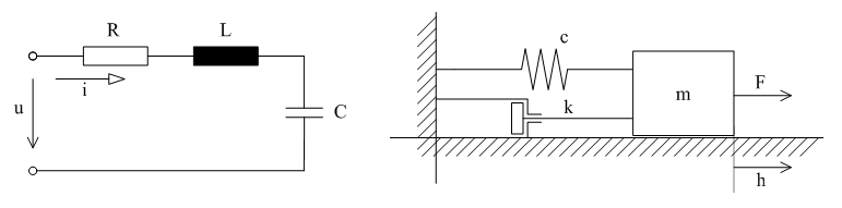
Figure 1: Analogous mechanical and electrical system

Electrical phenomena are analogous with fluid flow in many respects, so they can be illustrated by examining the characteristics of fluid flow.

The mathematical model describes the behaviour of the system with mathematical equations. It enables the analysis of system behaviour without the need to carry out experiments on the real system. We can use the system model to make calculations and numerically simulate the behaviour of the system. The system model is also used for designing controllers.

As an example, let’s see the mathematical description of the mechanical and electrical systems shown in Figure 1. The behaviour of the systems can be described with a differential equation which reveals the relationship between the input signal and its changes (derivatives) and the output signal and its changes (derivatives). Signals are quantities which have information content. The behaviour of the electrical system can be described with the following differential equation:

$u=iR+L\frac{di}{dt} +\frac{1}{C} \int _{0}^{t}id\tau $

This equation means that the sum of voltage drops on resistance, inductance and capacity gives the voltage fed into the network. The symbol of electric charge is q which is the integral of the electric current (this is taken here as an output signal). This way the above equation will take the following form:

$u=L\frac{d^{2} q}{dt^{2} } +R\frac{dq}{dt} +\frac{1}{C} q $

The differential equation of the mechanical system:

$F=m\frac{d^{2} h}{dt^{2} } +k\frac{dh}{dt} +ch $

which means that the resultant of the forces acting on the mass, which is the difference of the F tension force, the velocity-dependent fluid damping and the displacement-dependent spring force, results in the acceleration. It is clear from this that the behaviour of the electrical and that of the mechanical system is described by a second order differential equation. Analogous corresponding quantities in the two systems:

Now let’s mark the input signal with $u$, the output signal with $y$, and the parameter values with $a_{0} ,a_{1} ,a_{2} $. Both systems’ behaviour can be described with the following differential equation:

$a_{2} \frac{d^{2} y}{dt^{2} } +a_{1} \frac{dy}{dt} +a_{0} y=u $

A possible solution of the equation can be reached by expressing the highest differential coefficient (in the case of the mechanical system, the acceleration):

$\frac{d^{2} y}{dt^{2} } =\frac{1}{a_{2} } u-\frac{a_{1} }{a_{2} } \frac{dy}{dt} -\frac{a_{0} }{a_{2} } y $

The sudden change in the input signal only affects the acceleration first which, with the evolution of time, will change the velocity, and ultimately the displacement. (Velocity is shaped by the integration of the acceleration signal, while displacement is shaped by the integration of the velocity signal.)

Figure 2 shows the block diagram, which can be the basis of a calculation algorithm. By specifying the input signal and the initial conditions the integrator blocks calculate the derivative of the output signal and the change of the output signal versus time. (In the Figure the superscript in brackets indicate the derivatives.)

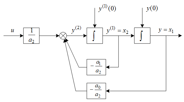Figure 2: Block diagram of the second order differential equation

The output signals of the integrators are important quantities for the system (displacement, velocity and electric charge, current) which are the so-called states of the system, their value is influenced by the earlier changes of the system, so we may say that they have a memory-like property. They are unable to immediately react to sudden input signal changes; they change gradually. With the state variables the second order differential equation can be transformed into a system of two first order differential equations. This is the so-called state equation of the system.

$\frac{dx_{1} }{dt} =x_{2}$

$\frac{dx_{2} }{dt} =-\frac{a_{0} }{a_{2} } x_{1} -\frac{a_{1} }{a_{2} } x_{2} +\frac{1}{a_{2} } u $

$y=x_{1} $

The model of the system makes it possible to examine and calculate the behaviour of the system, and its response to input signals and initial conditions. In simple cases (linear equations in the case of well-defined, analytically described input signals) the calculations can be performed analytically. These calculations are made easier by the various programming languages, such as Matlab, Mathematica and SIMUL for modelling or Prolog for logical relations.

References:

Levine (1996)

Szűcs (1970,1972)